A Tour of Machine Learning Algorithms
three different learning styles
1. Supervised Learning
2. Unsupervised Learning
3. Semi-Supervised Learning
Overview of Machine Learning Algorithms
Regression Algorithms
Instance-based Algorithms
Regularization Algorithms
Decision Tree Algorithms
Bayesian Algorithms
Clustering Algorithms
Association Rule Learning Algorithms
Artificial Neural Network Algorithms
Deep Learning Algorithms
Dimensionality Reduction Algorithms
Ensemble Algorithms
Other Machine Learning Algorithms
Other Lists of Machine Learning Algorithms
How to Study Machine Learning Algorithms
How to Run Machine Learning Algorithms
1.4 Install Packages
2.1 Load Data The Easy Way
2.2 Load From CSV
2.3. Create a Validation Dataset
3.1 Dimensions of Dataset
3.2 Types of Attributes
3.3 Peek at the Data
3.4 Levels of the Class
3.5 Class Distribution
3.6 Statistical Summary
4.1 Univariate Plots
4.2 Multivariate Plots
5.1 Test Harness
5.2 Build Models
5.3 Select Best Model
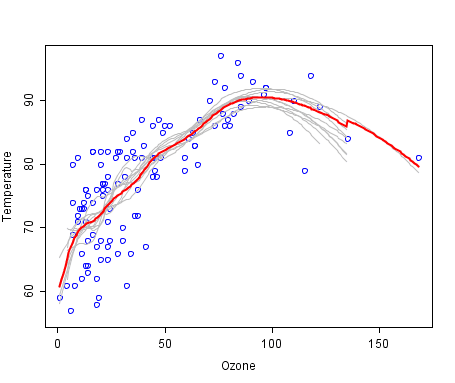 A cool example of an ensemble of lines of best fit.
Weak members are grey, the combined prediction is red.
Plot from Wikipedia, licensed under public domain.
A cool example of an ensemble of lines of best fit.
Weak members are grey, the combined prediction is red.
Plot from Wikipedia, licensed under public domain.
Algorithms Grouped by Learning Style
There are different ways an algorithm can model a problem based on its interaction with the experience or environment or whatever we want to call the input data.
It is popular in machine learning and artificial intelligence textbooks to first consider the learning styles that an algorithm can adopt.
There are only a few main learning styles or learning models that an algorithm can have and we'll go through them here with a few examples of algorithms and problem types that they suit.
This taxonomy or way of organizing machine learning algorithms is useful because it forces you to think about the roles of the input data and the model preparation process and select one that is the most appropriate for your problem in order to get the best result.
three different learning styles
1. Supervised Learning
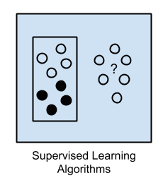 Input data is called training data and has a known label or result such as spam/not-spam or a stock price at a time.
A model is prepared through a training process in which it is required to make predictions and is corrected when those predictions are wrong.
The training process continues until the model achieves a desired level of accuracy on the training data.
Example problems are classification and regression.
Example algorithms include: Logistic Regression and the Back Propagation Neural Network.
Input data is called training data and has a known label or result such as spam/not-spam or a stock price at a time.
A model is prepared through a training process in which it is required to make predictions and is corrected when those predictions are wrong.
The training process continues until the model achieves a desired level of accuracy on the training data.
Example problems are classification and regression.
Example algorithms include: Logistic Regression and the Back Propagation Neural Network.
2. Unsupervised Learning
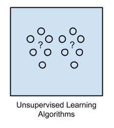 Input data is not labeled and does not have a known result.
A model is prepared by deducing structures present in the input data.
This may be to extract general rules.
It may be through a mathematical process to systematically reduce redundancy, or it may be to organize data by similarity.
Example problems are clustering, dimensionality reduction and association rule learning.
Example algorithms include: the Apriori algorithm and K-Means.
Input data is not labeled and does not have a known result.
A model is prepared by deducing structures present in the input data.
This may be to extract general rules.
It may be through a mathematical process to systematically reduce redundancy, or it may be to organize data by similarity.
Example problems are clustering, dimensionality reduction and association rule learning.
Example algorithms include: the Apriori algorithm and K-Means.
3. Semi-Supervised Learning
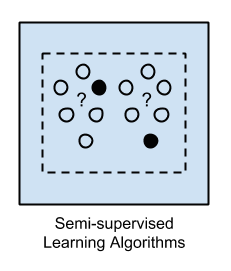 Input data is a mixture of labeled and unlabelled examples.
There is a desired prediction problem but the model must learn the structures to organize the data as well as make predictions.
Example problems are classification and regression.
Example algorithms are extensions to other flexible methods that make assumptions about how to model the unlabeled data.
Input data is a mixture of labeled and unlabelled examples.
There is a desired prediction problem but the model must learn the structures to organize the data as well as make predictions.
Example problems are classification and regression.
Example algorithms are extensions to other flexible methods that make assumptions about how to model the unlabeled data.
Overview of Machine Learning Algorithms
When crunching data to model business decisions, you are most typically using supervised and unsupervised learning methods. A hot topic at the moment is semi-supervised learning methods in areas such as image classification where there are large datasets with very few labeled examples.Algorithms Grouped By Similarity
Algorithms are often grouped by similarity in terms of their function (how they work).
For example, tree-based methods, and neural network inspired methods.
I think this is the most useful way to group algorithms and it is the approach we will use here.
This is a useful grouping method, but it is not perfect.
There are still algorithms that could just as easily fit into multiple categories like Learning Vector Quantization that is both a neural network inspired method and an instance-based method.
There are also categories that have the same name that describe the problem and the class of algorithm such as Regression and Clustering.
We could handle these cases by listing algorithms twice or by selecting the group that subjectively is the “best” fit.
I like this latter approach of not duplicating algorithms to keep things simple.
In this section, we list many of the popular machine learning algorithms grouped the way we think is the most intuitive.
The list is not exhaustive in either the groups or the algorithms, but I think it is representative and will be useful to you to get an idea of the lay of the land.
Please Note: There is a strong bias towards algorithms used for classification and regression, the two most prevalent supervised machine learning problems you will encounter.
If you know of an algorithm or a group of algorithms not listed, put it in the comments and share it with us.
Let's dive in.
Regression Algorithms
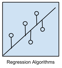 Regression is concerned with modeling the relationship between variables that is iteratively refined using a measure of error in the predictions made by the model.
Regression methods are a workhorse of statistics and have been co-opted into statistical machine learning.
This may be confusing because we can use regression to refer to the class of problem and the class of algorithm.
Really, regression is a process.
The most popular regression algorithms are:
Ordinary Least Squares Regression (OLSR)
Linear Regression
Logistic Regression
Stepwise Regression
Multivariate Adaptive Regression Splines (MARS)
Locally Estimated Scatterplot Smoothing (LOESS)
Regression is concerned with modeling the relationship between variables that is iteratively refined using a measure of error in the predictions made by the model.
Regression methods are a workhorse of statistics and have been co-opted into statistical machine learning.
This may be confusing because we can use regression to refer to the class of problem and the class of algorithm.
Really, regression is a process.
The most popular regression algorithms are:
Ordinary Least Squares Regression (OLSR)
Linear Regression
Logistic Regression
Stepwise Regression
Multivariate Adaptive Regression Splines (MARS)
Locally Estimated Scatterplot Smoothing (LOESS)
Instance-based Algorithms
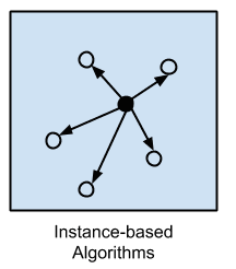 Instance-based learning model is a decision problem with instances or examples of training data that are deemed important or required to the model.
Such methods typically build up a database of example data and compare new data to the database using a similarity measure in order to find the best match and make a prediction.
For this reason, instance-based methods are also called winner-take-all methods and memory-based learning.
Focus is put on the representation of the stored instances and similarity measures used between instances.
The most popular instance-based algorithms are:
k-Nearest Neighbor (kNN)
Learning Vector Quantization (LVQ)
Self-Organizing Map (SOM)
Locally Weighted Learning (LWL)
Support Vector Machines (SVM)
Instance-based learning model is a decision problem with instances or examples of training data that are deemed important or required to the model.
Such methods typically build up a database of example data and compare new data to the database using a similarity measure in order to find the best match and make a prediction.
For this reason, instance-based methods are also called winner-take-all methods and memory-based learning.
Focus is put on the representation of the stored instances and similarity measures used between instances.
The most popular instance-based algorithms are:
k-Nearest Neighbor (kNN)
Learning Vector Quantization (LVQ)
Self-Organizing Map (SOM)
Locally Weighted Learning (LWL)
Support Vector Machines (SVM)
Regularization Algorithms
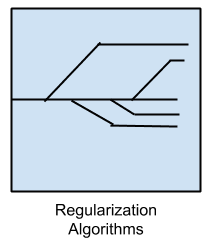 An extension made to another method (typically regression methods) that penalizes models based on their complexity, favoring simpler models that are also better at generalizing.
I have listed regularization algorithms separately here because they are popular, powerful and generally simple modifications made to other methods.
The most popular regularization algorithms are:
Ridge Regression
Least Absolute Shrinkage and Selection Operator (LASSO)
Elastic Net
Least-Angle Regression (LARS)
An extension made to another method (typically regression methods) that penalizes models based on their complexity, favoring simpler models that are also better at generalizing.
I have listed regularization algorithms separately here because they are popular, powerful and generally simple modifications made to other methods.
The most popular regularization algorithms are:
Ridge Regression
Least Absolute Shrinkage and Selection Operator (LASSO)
Elastic Net
Least-Angle Regression (LARS)
Decision Tree Algorithms
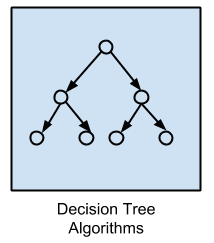 Decision tree methods construct a model of decisions made based on actual values of attributes in the data.
Decisions fork in tree structures until a prediction decision is made for a given record.
Decision trees are trained on data for classification and regression problems.
Decision trees are often fast and accurate and a big favorite in machine learning.
The most popular decision tree algorithms are:
Classification and Regression Tree (CART)
Iterative Dichotomiser 3 (ID3)
C4.5 and C5.0 (different versions of a powerful approach)
Chi-squared Automatic Interaction Detection (CHAID)
Decision Stump
M5
Conditional Decision Trees
Decision tree methods construct a model of decisions made based on actual values of attributes in the data.
Decisions fork in tree structures until a prediction decision is made for a given record.
Decision trees are trained on data for classification and regression problems.
Decision trees are often fast and accurate and a big favorite in machine learning.
The most popular decision tree algorithms are:
Classification and Regression Tree (CART)
Iterative Dichotomiser 3 (ID3)
C4.5 and C5.0 (different versions of a powerful approach)
Chi-squared Automatic Interaction Detection (CHAID)
Decision Stump
M5
Conditional Decision Trees
Bayesian Algorithms
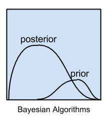 Bayesian methods are those that explicitly apply Bayes' Theorem for problems such as classification and regression.
The most popular Bayesian algorithms are:
Naive Bayes
Gaussian Naive Bayes
Multinomial Naive Bayes
Averaged One-Dependence Estimators (AODE)
Bayesian Belief Network (BBN)
Bayesian Network (BN)
Bayesian methods are those that explicitly apply Bayes' Theorem for problems such as classification and regression.
The most popular Bayesian algorithms are:
Naive Bayes
Gaussian Naive Bayes
Multinomial Naive Bayes
Averaged One-Dependence Estimators (AODE)
Bayesian Belief Network (BBN)
Bayesian Network (BN)
Clustering Algorithms
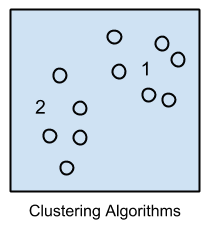 Clustering, like regression, describes the class of problem and the class of methods.
Clustering methods are typically organized by the modeling approaches such as centroid-based and hierarchal.
All methods are concerned with using the inherent structures in the data to best organize the data into groups of maximum commonality.
The most popular clustering algorithms are:
k-Means
k-Medians
Expectation Maximisation (EM)
Hierarchical Clustering
Clustering, like regression, describes the class of problem and the class of methods.
Clustering methods are typically organized by the modeling approaches such as centroid-based and hierarchal.
All methods are concerned with using the inherent structures in the data to best organize the data into groups of maximum commonality.
The most popular clustering algorithms are:
k-Means
k-Medians
Expectation Maximisation (EM)
Hierarchical Clustering
Association Rule Learning Algorithms
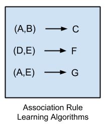 Association rule learning methods extract rules that best explain observed relationships between variables in data.
These rules can discover important and commercially useful associations in large multidimensional datasets that can be exploited by an organization.
The most popular association rule learning algorithms are:
Apriori algorithm
Eclat algorithm
Association rule learning methods extract rules that best explain observed relationships between variables in data.
These rules can discover important and commercially useful associations in large multidimensional datasets that can be exploited by an organization.
The most popular association rule learning algorithms are:
Apriori algorithm
Eclat algorithm
Artificial Neural Network Algorithms
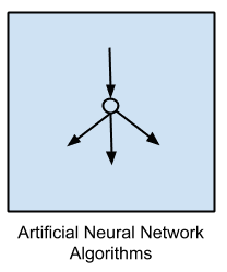 Artificial Neural Networks are models that are inspired by the structure and/or function of biological neural networks.
They are a class of pattern matching that are commonly used for regression and classification problems but are really an enormous subfield comprised of hundreds of algorithms and variations for all manner of problem types.
Note that I have separated out Deep Learning from neural networks because of the massive growth and popularity in the field.
Here we are concerned with the more classical methods.
The most popular artificial neural network algorithms are:
Perceptron
Multilayer Perceptrons (MLP)
Back-Propagation
Stochastic Gradient Descent
Hopfield Network
Radial Basis Function Network (RBFN)
Artificial Neural Networks are models that are inspired by the structure and/or function of biological neural networks.
They are a class of pattern matching that are commonly used for regression and classification problems but are really an enormous subfield comprised of hundreds of algorithms and variations for all manner of problem types.
Note that I have separated out Deep Learning from neural networks because of the massive growth and popularity in the field.
Here we are concerned with the more classical methods.
The most popular artificial neural network algorithms are:
Perceptron
Multilayer Perceptrons (MLP)
Back-Propagation
Stochastic Gradient Descent
Hopfield Network
Radial Basis Function Network (RBFN)
Deep Learning Algorithms
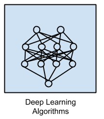 Deep Learning methods are a modern update to Artificial Neural Networks that exploit abundant cheap computation.
They are concerned with building much larger and more complex neural networks and, as commented on above, many methods are concerned with very large datasets of labelled analog data, such as image, text.
audio, and video.
The most popular deep learning algorithms are:
Convolutional Neural Network (CNN)
Recurrent Neural Networks (RNNs)
Long Short-Term Memory Networks (LSTMs)
Stacked Auto-Encoders
Deep Boltzmann Machine (DBM)
Deep Belief Networks (DBN)
Deep Learning methods are a modern update to Artificial Neural Networks that exploit abundant cheap computation.
They are concerned with building much larger and more complex neural networks and, as commented on above, many methods are concerned with very large datasets of labelled analog data, such as image, text.
audio, and video.
The most popular deep learning algorithms are:
Convolutional Neural Network (CNN)
Recurrent Neural Networks (RNNs)
Long Short-Term Memory Networks (LSTMs)
Stacked Auto-Encoders
Deep Boltzmann Machine (DBM)
Deep Belief Networks (DBN)
Dimensionality Reduction Algorithms
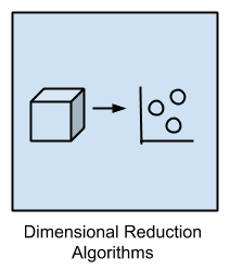 Like clustering methods, dimensionality reduction seek and exploit the inherent structure in the data, but in this case in an unsupervised manner or order to summarize or describe data using less information.
This can be useful to visualize dimensional data or to simplify data which can then be used in a supervised learning method.
Many of these methods can be adapted for use in classification and regression.
Principal Component Analysis (PCA)
Principal Component Regression (PCR)
Partial Least Squares Regression (PLSR)
Sammon Mapping
Multidimensional Scaling (MDS)
Projection Pursuit
Linear Discriminant Analysis (LDA)
Mixture Discriminant Analysis (MDA)
Quadratic Discriminant Analysis (QDA)
Flexible Discriminant Analysis (FDA)
Like clustering methods, dimensionality reduction seek and exploit the inherent structure in the data, but in this case in an unsupervised manner or order to summarize or describe data using less information.
This can be useful to visualize dimensional data or to simplify data which can then be used in a supervised learning method.
Many of these methods can be adapted for use in classification and regression.
Principal Component Analysis (PCA)
Principal Component Regression (PCR)
Partial Least Squares Regression (PLSR)
Sammon Mapping
Multidimensional Scaling (MDS)
Projection Pursuit
Linear Discriminant Analysis (LDA)
Mixture Discriminant Analysis (MDA)
Quadratic Discriminant Analysis (QDA)
Flexible Discriminant Analysis (FDA)
Ensemble Algorithms
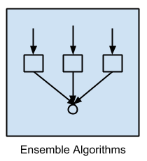 Ensemble methods are models composed of multiple weaker models that are independently trained and whose predictions are combined in some way to make the overall prediction.
Much effort is put into what types of weak learners to combine and the ways in which to combine them.
This is a very powerful class of techniques and as such is very popular.
Boosting
Bootstrapped Aggregation (Bagging)
AdaBoost
Weighted Average (Blending)
Stacked Generalization (Stacking)
Gradient Boosting Machines (GBM)
Gradient Boosted Regression Trees (GBRT)
Random Forest
Ensemble methods are models composed of multiple weaker models that are independently trained and whose predictions are combined in some way to make the overall prediction.
Much effort is put into what types of weak learners to combine and the ways in which to combine them.
This is a very powerful class of techniques and as such is very popular.
Boosting
Bootstrapped Aggregation (Bagging)
AdaBoost
Weighted Average (Blending)
Stacked Generalization (Stacking)
Gradient Boosting Machines (GBM)
Gradient Boosted Regression Trees (GBRT)
Random Forest
Other Machine Learning Algorithms
Many algorithms were not covered. I did not cover algorithms from specialty tasks in the process of machine learning, such as: Feature selection algorithms Algorithm accuracy evaluation Performance measures Optimization algorithms I also did not cover algorithms from specialty subfields of machine learning, such as: Computational intelligence (evolutionary algorithms, etc.) Computer Vision (CV) Natural Language Processing (NLP) Recommender Systems Reinforcement Learning Graphical Models And more… These may feature in future posts.Further Reading on Machine Learning Algorithms
This tour of machine learning algorithms was intended to give you an overview of what is out there and some ideas on how to relate algorithms to each other.
I've collected together some resources for you to continue your reading on algorithms.
If you have a specific question, please leave a comment.
Other Lists of Machine Learning Algorithms
There are other great lists of algorithms out there if you're interested. Below are few hand selected examples. List of Machine Learning Algorithms: On Wikipedia. Although extensive, I do not find this list or the organization of the algorithms particularly useful. Machine Learning Algorithms Category: Also on Wikipedia, slightly more useful than Wikipedias great list above. It organizes algorithms alphabetically. CRAN Task View: Machine Learning & Statistical Learning: A list of all the packages and all the algorithms supported by each machine learning package in R. Gives you a grounded feeling of what's out there and what people are using for analysis day-to-day. Top 10 Algorithms in Data Mining: Published article and now a book (Affiliate Link) on the most popular algorithms for data mining. Another grounded and less overwhelming take on methods that you could go off and learn deeply.How to Study Machine Learning Algorithms
Algorithms are a big part of machine learning. It's a topic I am passionate about and write about a lot on this blog. Below are few hand selected posts that might interest you for further reading. How to Learn Any Machine Learning Algorithm: A systematic approach that you can use to study and understand any machine learning algorithm using “algorithm description templates” (I used this approach to write my first book). How to Create Targeted Lists of Machine Learning Algorithms: How you can create your own systematic lists of machine learning algorithms to jump start work on your next machine learning problem. How to Research a Machine Learning Algorithm: A systematic approach that you can use to research machine learning algorithms (works great in collaboration with the template approach listed above). How to Investigate Machine Learning Algorithm Behavior: A methodology you can use to understand how machine learning algorithms work by creating and executing very small studies into their behavior. Research is not just for academics! How to Implement a Machine Learning Algorithm: A process and tips and tricks for implementing machine learning algorithms from scratch.How to Run Machine Learning Algorithms
Sometimes you just want to dive into code. Below are some links you can use to run machine learning algorithms, code them up using standard libraries or implement them from scratch. How To Get Started With Machine Learning Algorithms in R: Links to a large number of code examples on this site demonstrating machine learning algorithms in R. Machine Learning Algorithm Recipes in scikit-learn: A collection of Python code examples demonstrating how to create predictive models using scikit-learn. How to Run Your First Classifier in Weka: A tutorial for running your very first classifier in Weka (no code required!).Machine Learning in R
https://machinelearningmastery.com/machine-learning-in-r-step-by-step/
1.4 Install Packages
install.packages("caret") UPDATE: We may need other packages, but caret should ask us if we want to load them. If you are having problems with packages, you can install the caret packages and all packages that you might need by typing: install.packages("caret", dependencies=c("Depends", "Suggests")) Now, let's load the package that we are going to use in this tutorial, the caret package. library(caret) The caret package provides a consistent interface into hundreds of machine learning algorithms and provides useful convenience methods for data visualization, data resampling, model tuning and model comparison, among other features. It's a must have tool for machine learning projects in R. For more information about the caret R package see the caret package homepage.2. Load The Data
We are going to use the iris flowers dataset.
This dataset is famous because it is used as the "hello world" dataset in machine learning and statistics by pretty much everyone.
The dataset contains 150 observations of iris flowers.
There are four columns of measurements of the flowers in centimeters.
The fifth column is the species of the flower observed.
All observed flowers belong to one of three species.
You can learn more about this dataset on Wikipedia.
Here is what we are going to do in this step:
Load the iris data the easy way.
Load the iris data from CSV (optional, for purists).
Separate the data into a training dataset and a validation dataset.
Choose your preferred way to load data or try both methods.
2.1 Load Data The Easy Way
Fortunately, the R platform provides the iris dataset for us. Load the dataset as follows: # attach the iris dataset to the environment data(iris) # rename the dataset dataset <- iris You now have the iris data loaded in R and accessible via the dataset variable. I like to name the loaded data "dataset". This is helpful if you want to copy-paste code between projects and the dataset always has the same name.2.2 Load From CSV
Maybe your a purist and you want to load the data just like you would on your own machine learning project, from a CSV file. Download the iris dataset from the UCI Machine Learning Repository (here is the direct link). Save the file as iris.csv your project directory. Load the dataset from the CSV file as follows: # define the filename filename <- "iris.csv" # load the CSV file from the local directory dataset <- read.csv(filename, header=FALSE) # set the column names in the dataset colnames(dataset) <- c("Sepal.Length","Sepal.Width","Petal.Length","Petal.Width","Species") You now have the iris data loaded in R and accessible via the dataset variable.2.3. Create a Validation Dataset
We need to know that the model we created is any good. Later, we will use statistical methods to estimate the accuracy of the models that we create on unseen data. We also want a more concrete estimate of the accuracy of the best model on unseen data by evaluating it on actual unseen data. That is, we are going to hold back some data that the algorithms will not get to see and we will use this data to get a second and independent idea of how accurate the best model might actually be. We will split the loaded dataset into two, 80% of which we will use to train our models and 20% that we will hold back as a validation dataset. # create a list of 80% of the rows in the original dataset we can use for training validation_index <- createDataPartition(dataset$Species, p=0.80, list=FALSE) # select 20% of the data for validation validation <- dataset[-validation_index,] # use the remaining 80% of data to training and testing the models dataset <- dataset[validation_index,] You now have training data in the dataset variable and a validation set we will use later in the validation variable. Note that we replaced our dataset variable with the 80% sample of the dataset. This was an attempt to keep the rest of the code simpler and readable.3. Summarize Dataset
Now it is time to take a look at the data.
In this step we are going to take a look at the data a few different ways:
Dimensions of the dataset.
Types of the attributes.
Peek at the data itself.
Levels of the class attribute.
Breakdown of the instances in each class.
Statistical summary of all attributes.
Don't worry, each look at the data is one command.
These are useful commands that you can use again and again on future projects.
3.1 Dimensions of Dataset
We can get a quick idea of how many instances (rows) and how many attributes (columns) the data contains with the dim function. # dimensions of dataset dim(dataset) You should see 120 instances and 5 attributes: [1] 120 53.2 Types of Attributes
It is a good idea to get an idea of the types of the attributes. They could be doubles, integers, strings, factors and other types. Knowing the types is important as it will give you an idea of how to better summarize the data you have and the types of transforms you might need to use to prepare the data before you model it. # list types for each attribute sapply(dataset, class) You should see that all of the inputs are double and that the class value is a factor: Sepal.Length Sepal.Width Petal.Length Petal.Width Species "numeric" "numeric" "numeric" "numeric" "factor"3.3 Peek at the Data
It is also always a good idea to actually eyeball your data. # take a peek at the first 5 rows of the data head(dataset) You should see the first 5 rows of the data: Sepal.Length Sepal.Width Petal.Length Petal.Width Species 1 5.1 3.5 1.4 0.2 setosa 2 4.9 3.0 1.4 0.2 setosa 3 4.7 3.2 1.3 0.2 setosa 5 5.0 3.6 1.4 0.2 setosa 6 5.4 3.9 1.7 0.4 setosa 7 4.6 3.4 1.4 0.3 setosa3.4 Levels of the Class
The class variable is a factor. A factor is a class that has multiple class labels or levels. Let's look at the levels: # list the levels for the class levels(dataset$Species) Notice above how we can refer to an attribute by name as a property of the dataset. In the results we can see that the class has 3 different labels: [1] "setosa" "versicolor" "virginica" This is a multi-class or a multinomial classification problem. If there were two levels, it would be a binary classification problem.3.5 Class Distribution
Let's now take a look at the number of instances (rows) that belong to each class. We can view this as an absolute count and as a percentage. # summarize the class distribution percentage <- prop.table(table(dataset$Species)) * 100 cbind(freq=table(dataset$Species), percentage=percentage) We can see that each class has the same number of instances (40 or 33% of the dataset) freq percentage setosa 40 33.33333 versicolor 40 33.33333 virginica 40 33.333333.6 Statistical Summary
Now finally, we can take a look at a summary of each attribute. This includes the mean, the min and max values as well as some percentiles (25th, 50th or media and 75th e.g. values at this points if we ordered all the values for an attribute). # summarize attribute distributions summary(dataset) We can see that all of the numerical values have the same scale (centimeters) and similar ranges [0,8] centimeters. Sepal.Length Sepal.Width Petal.Length Petal.Width Species Min. :4.300 Min. :2.00 Min. :1.000 Min. :0.100 setosa :40 1st Qu.:5.100 1st Qu.:2.80 1st Qu.:1.575 1st Qu.:0.300 versicolor:40 Median :5.800 Median :3.00 Median :4.300 Median :1.350 virginica :40 Mean :5.834 Mean :3.07 Mean :3.748 Mean :1.213 3rd Qu.:6.400 3rd Qu.:3.40 3rd Qu.:5.100 3rd Qu.:1.800 Max. :7.900 Max. :4.40 Max. :6.900 Max. :2.5004. Visualize Dataset
We now have a basic idea about the data.
We need to extend that with some visualizations.
We are going to look at two types of plots:
Univariate plots to better understand each attribute.
Multivariate plots to better understand the relationships between attributes.
4.1 Univariate Plots
We start with some univariate plots, that is, plots of each individual variable. It is helpful with visualization to have a way to refer to just the input attributes and just the output attributes. Let's set that up and call the inputs attributes x and the output attribute (or class) y. # split input and output x <- dataset[,1:4] y <- dataset[,5] Given that the input variables are numeric, we can create box and whisker plots of each. # boxplot for each attribute on one image par(mfrow=c(1,4)) for(i in 1:4) { boxplot(x[,i], main=names(iris)[i]) } This gives us a much clearer idea of the distribution of the input attributes: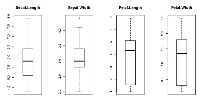 Box and Whisker Plots in R
We can also create a barplot of the Species class variable to get a graphical representation of the class distribution (generally uninteresting in this case because they're even).
# barplot for class breakdown
plot(y)
This confirms what we learned in the last section, that the instances are evenly distributed across the three class:
Box and Whisker Plots in R
We can also create a barplot of the Species class variable to get a graphical representation of the class distribution (generally uninteresting in this case because they're even).
# barplot for class breakdown
plot(y)
This confirms what we learned in the last section, that the instances are evenly distributed across the three class:
 Bar Plot of Iris Flower Species
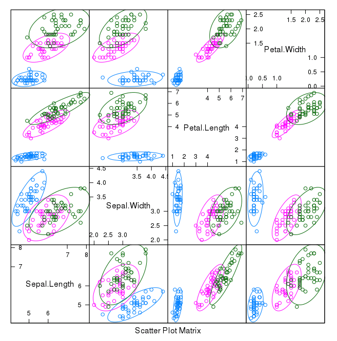
4.2 Multivariate Plots
Now we can look at the interactions between the variables. First let's look at scatterplots of all pairs of attributes and color the points by class. In addition, because the scatterplots show that points for each class are generally separate, we can draw ellipses around them. # scatterplot matrix featurePlot(x=x, y=y, plot="ellipse") We can see some clear relationships between the input attributes (trends) and between attributes and the class values (ellipses):
Scatterplot Matrix of Iris Data in R
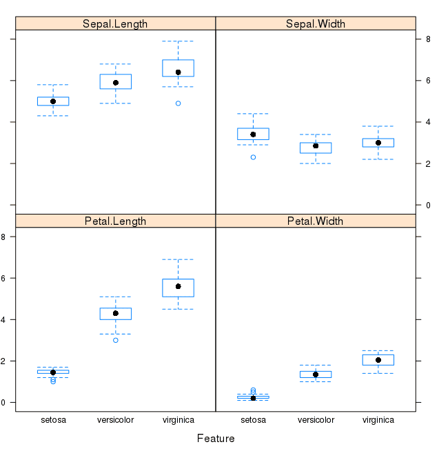
We can also look at box and whisker plots of each input variable again, but this time broken down into separate plots for each class.
This can help to tease out obvious linear separations between the classes.
# box and whisker plots for each attribute
featurePlot(x=x, y=y, plot="box")
This is useful to see that there are clearly different distributions of the attributes for each class value.
 Box and Whisker Plot of Iris data by Class Value
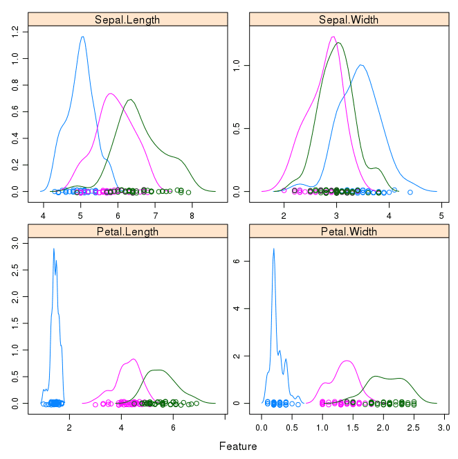
Next we can get an idea of the distribution of each attribute, again like the box and whisker plots, broken down by class value.
Sometimes histograms are good for this, but in this case we will use some probability density plots to give nice smooth lines for each distribution.
# density plots for each attribute by class value
scales <- list(x=list(relation="free"), y=list(relation="free"))
featurePlot(x=x, y=y, plot="density", scales=scales)
Like the boxplots, we can see the difference in distribution of each attribute by class value.
We can also see the Gaussian-like distribution (bell curve) of each attribute.
Box and Whisker Plot of Iris data by Class Value
Next we can get an idea of the distribution of each attribute, again like the box and whisker plots, broken down by class value.
Sometimes histograms are good for this, but in this case we will use some probability density plots to give nice smooth lines for each distribution.
# density plots for each attribute by class value
scales <- list(x=list(relation="free"), y=list(relation="free"))
featurePlot(x=x, y=y, plot="density", scales=scales)
Like the boxplots, we can see the difference in distribution of each attribute by class value.
We can also see the Gaussian-like distribution (bell curve) of each attribute.
 Density Plots of Iris Data By Class Value
5. Evaluate Some Algorithms
Now it is time to create some models of the data and estimate their accuracy on unseen data.
Here is what we are going to cover in this step:
Set-up the test harness to use 10-fold cross validation.
Build 5 different models to predict species from flower measurements
Select the best model.
5.1 Test Harness
We will 10-fold crossvalidation to estimate accuracy. This will split our dataset into 10 parts, train in 9 and test on 1 and release for all combinations of train-test splits. We will also repeat the process 3 times for each algorithm with different splits of the data into 10 groups, in an effort to get a more accurate estimate. # Run algorithms using 10-fold cross validation control <- trainControl(method="cv", number=10) metric <- "Accuracy" We are using the metric of "Accuracy" to evaluate models. This is a ratio of the number of correctly predicted instances in divided by the total number of instances in the dataset multiplied by 100 to give a percentage (e.g. 95% accurate). We will be using the metric variable when we run build and evaluate each model next.5.2 Build Models
We don't know which algorithms would be good on this problem or what configurations to use. We get an idea from the plots that some of the classes are partially linearly separable in some dimensions, so we are expecting generally good results. Let's evaluate 5 different algorithms: Linear Discriminant Analysis (LDA) Classification and Regression Trees (CART). k-Nearest Neighbors (kNN). Support Vector Machines (SVM) with a linear kernel. Random Forest (RF) This is a good mixture of simple linear (LDA), nonlinear (CART, kNN) and complex nonlinear methods (SVM, RF). We reset the random number seed before reach run to ensure that the evaluation of each algorithm is performed using exactly the same data splits. It ensures the results are directly comparable. Let's build our five models: # a) linear algorithms set.seed(7) fit.lda <- train(Species~., data=dataset, method="lda", metric=metric, trControl=control) # b) nonlinear algorithms # CART set.seed(7) fit.cart <- train(Species~., data=dataset, method="rpart", metric=metric, trControl=control) # kNN set.seed(7) fit.knn <- train(Species~., data=dataset, method="knn", metric=metric, trControl=control) # c) advanced algorithms # SVM set.seed(7) fit.svm <- train(Species~., data=dataset, method="svmRadial", metric=metric, trControl=control) # Random Forest set.seed(7) fit.rf <- train(Species~., data=dataset, method="rf", metric=metric, trControl=control) Caret does support the configuration and tuning of the configuration of each model, but we are not going to cover that in this tutorial.5.3 Select Best Model
We now have 5 models and accuracy estimations for each. We need to compare the models to each other and select the most accurate. We can report on the accuracy of each model by first creating a list of the created models and using the summary function. # summarize accuracy of models results <- resamples(list(lda=fit.lda, cart=fit.cart, knn=fit.knn, svm=fit.svm, rf=fit.rf)) summary(results) We can see the accuracy of each classifier and also other metrics like Kappa: Models: lda, cart, knn, svm, rf Number of resamples: 10 Accuracy Min. 1st Qu. Median Mean 3rd Qu. Max. NA's lda 0.9167 0.9375 1.0000 0.9750 1 1 0 cart 0.8333 0.9167 0.9167 0.9417 1 1 0 knn 0.8333 0.9167 1.0000 0.9583 1 1 0 svm 0.8333 0.9167 0.9167 0.9417 1 1 0 rf 0.8333 0.9167 0.9583 0.9500 1 1 0 Kappa Min. 1st Qu. Median Mean 3rd Qu. Max. NA's lda 0.875 0.9062 1.0000 0.9625 1 1 0 cart 0.750 0.8750 0.8750 0.9125 1 1 0 knn 0.750 0.8750 1.0000 0.9375 1 1 0 svm 0.750 0.8750 0.8750 0.9125 1 1 0 rf 0.750 0.8750 0.9375 0.9250 1 1 0 We can also create a plot of the model evaluation results and compare the spread and the mean accuracy of each model. There is a population of accuracy measures for each algorithm because each algorithm was evaluated 10 times (10 fold cross validation). # compare accuracy of models dotplot(results) We can see that the most accurate model in this case was LDA: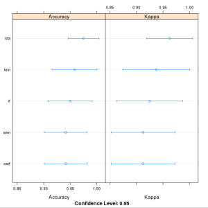 Comparison of Machine Learning Algorithms on Iris Dataset in R
The results for just the LDA model can be summarized.
# summarize Best Model
print(fit.lda)
This gives a nice summary of what was used to train the model and the mean and standard deviation (SD) accuracy achieved, specifically 97.5% accuracy +/- 4%
Linear Discriminant Analysis
120 samples
4 predictor
3 classes: 'setosa', 'versicolor', 'virginica'
No pre-processing
Resampling: Cross-Validated (10 fold)
Summary of sample sizes: 108, 108, 108, 108, 108, 108, ...
Resampling results
Accuracy Kappa Accuracy SD Kappa SD
0.975 0.9625 0.04025382 0.06038074
Comparison of Machine Learning Algorithms on Iris Dataset in R
The results for just the LDA model can be summarized.
# summarize Best Model
print(fit.lda)
This gives a nice summary of what was used to train the model and the mean and standard deviation (SD) accuracy achieved, specifically 97.5% accuracy +/- 4%
Linear Discriminant Analysis
120 samples
4 predictor
3 classes: 'setosa', 'versicolor', 'virginica'
No pre-processing
Resampling: Cross-Validated (10 fold)
Summary of sample sizes: 108, 108, 108, 108, 108, 108, ...
Resampling results
Accuracy Kappa Accuracy SD Kappa SD
0.975 0.9625 0.04025382 0.06038074
6. Make Predictions
The LDA was the most accurate model.
Now we want to get an idea of the accuracy of the model on our validation set.
This will give us an independent final check on the accuracy of the best model.
It is valuable to keep a validation set just in case you made a slip during such as overfitting to the training set or a data leak.
Both will result in an overly optimistic result.
We can run the LDA model directly on the validation set and summarize the results in a confusion matrix.
# estimate skill of LDA on the validation dataset
predictions <- predict(fit.lda, validation)
confusionMatrix(predictions, validation$Species)
We can see that the accuracy is 100%.
It was a small validation dataset (20%), but this result is within our expected margin of 97% +/-4% suggesting we may have an accurate and a reliably accurate model.
Confusion Matrix and Statistics
Reference
Prediction setosa versicolor virginica
setosa 10 0 0
versicolor 0 10 0
virginica 0 0 10
Overall Statistics
Accuracy : 1
95% CI : (0.8843, 1)
No Information Rate : 0.3333
P-Value [Acc > NIR] : 4.857e-15
Kappa : 1
Mcnemar's Test P-Value : NA
Statistics by Class:
Class: setosa Class: versicolor Class: virginica
Sensitivity 1.0000 1.0000 1.0000
Specificity 1.0000 1.0000 1.0000
Pos Pred Value 1.0000 1.0000 1.0000
Neg Pred Value 1.0000 1.0000 1.0000
Prevalence 0.3333 0.3333 0.3333
Detection Rate 0.3333 0.3333 0.3333
Detection Prevalence 0.3333 0.3333 0.3333
Balanced Accuracy 1.0000 1.0000 1.0000
You Can Do Machine Learning in R
Work through the tutorial above.
It will take you 5-to-10 minutes, max!
You do not need to understand everything.
(at least not right now) Your goal is to run through the tutorial end-to-end and get a result.
You do not need to understand everything on the first pass.
List down your questions as you go.
Make heavy use of the ?FunctionName help syntax in R to learn about all of the functions that you're using.
You do not need to know how the algorithms work.
It is important to know about the limitations and how to configure machine learning algorithms.
But learning about algorithms can come later.
You need to build up this algorithm knowledge slowly over a long period of time.
Today, start off by getting comfortable with the platform.
You do not need to be an R programmer.
The syntax of the R language can be confusing.
Just like other languages, focus on function calls (e.g.
function()) and assignments (e.g.
a <- "b").
This will get you most of the way.
You are a developer, you know how to pick up the basics of a language real fast.
Just get started and dive into the details later.
You do not need to be a machine learning expert.
You can learn about the benefits and limitations of various algorithms later, and there are plenty of posts that you can read later to brush up on the steps of a machine learning project and the importance of evaluating accuracy using cross validation.
What about other steps in a machine learning project.
We did not cover all of the steps in a machine learning project because this is your first project and we need to focus on the key steps.
Namely, loading data, looking at the data, evaluating some algorithms and making some predictions.
In later tutorials we can look at other data preparation and result improvement tasks.
Summary
In this post you discovered step-by-step how to complete your first machine learning project in R.
You discovered that completing a small end-to-end project from loading the data to making predictions is the best way to get familiar with a new platform.
Example
Using AI to classify and grade human mood
This can be approached as a machine learning problem.
Here's a general outline of the steps:
Gather and prepare a dataset:
Collect a dataset of labeled examples where human moods are classified and graded.
You can use surveys, self-reporting tools, or other methods to gather mood data.
Make sure the dataset is diverse and representative of different moods.
Define the mood categories and grading system:
Determine the mood categories you want to classify and the grading system you want to use.
For example, you might have categories like happy, sad, angry, etc., and a grading system from 1 to 5.
Feature extraction:
Extract relevant features from the dataset that can help in predicting mood.
These features could include facial expressions, voice tone, text sentiment, physiological signals, or any other relevant data.
Preprocessing and normalizing the features might be necessary.
Select a machine learning model:
Choose an appropriate machine learning model for mood classification and grading.
Options include decision trees, random forests, support vector machines (SVM), or deep learning models like convolutional neural networks (CNNs) or recurrent neural networks (RNNs).
Train the model:
Split your dataset into training and validation sets.
Use the training set to train your chosen machine learning model.
The model will learn the patterns and relationships between the features and mood labels.
Evaluate and fine-tune the model:
Evaluate your model's performance on the validation set using appropriate evaluation metrics, such as accuracy, precision, recall, or F1-score.
If the performance is not satisfactory, consider fine-tuning the model by adjusting hyperparameters, trying different algorithms, or increasing the dataset size.
Test the model:
Once you are satisfied with the model's performance, test it on a separate test set that was not used during training or validation.
This will give you an unbiased estimate of how well the model generalizes to unseen data.
Deploy the model:
Once the model performs well on the test set, you can deploy it in a production environment.
This could be a mobile app, a web application, or any other platform where you want to classify and grade human mood.
Continuously improve the model:
Collect feedback from users and update your model periodically to improve its performance.
This could involve retraining the model with new data or incorporating new features.
Remember, the accuracy and reliability of the mood classification and grading system heavily depend on the quality and representativeness of the dataset, as well as the chosen machine learning model.
Ensemble 全体 整体 methods: bagging, boosting and stacking
Introduction
Outline
What are ensemble methods?
Single weak learner
Combine weak learners
Focus on bagging
Bootstrapping
Focus on boosting
Boosting
Gradient boosting
Overview of stacking
Stacking
Takeaways
Outline
What are ensemble methods?
Single weak learner
Combine weak learners
Focus on bagging
Bootstrapping
Focus on boosting
Boosting
Gradient boosting
Overview of stacking
Stacking
Takeaways